In stage 2 we get the quiz to mark the questions, there are several ways to do this however for this tutorial I am going to use an IF statement. This allows us to have two responses, correct and incorrect, these can be substituted for your own message.
I am going to have the answer in cell B4 and the responce in B5, so the code for B5 is
=IF(B4="Johnny Depp", "Correct", "Wrong")
the italicised parts are the ones you will have to change for each picture.
B4 - the cell reference for the answer you are checking.
"Johnny Depp" - the correct answer.
It is important to note that for the counter I am going to create later to work the 'correct' message must be the same for every picture.
Set the answer cells to change colour using conditional formatting, in Office 2007 this is to the right on the home tab.
Simply set the cell to change colour when the cell is equal to your 'correct' message.
Saturday, 20 March 2010
Excel Picture Quiz
So I thought it was about time I put something on here and I thought what better than to start with some instructions for creating a simple and fun picture quiz in Excel.
The instructions presume you have some basic knowledge of Excel to start with, but if there are any steps which you want explaining in more detail feel free to contact me using the quick contact on my website www.zypher.co.uk
I will split this into the following stages / lessons
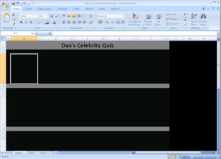
Next set the height of some of the rows to allow them to hold the images, leaving at least 2 rows normal height, this is where the answer and correct or incorrect message will go.
Set the background colour of the cells and add a title to the centre of your top row.
Insert your images into the larger cells and add instructions to the side, I have used a text box though you could just as easily merge some cells for this.
The instructions presume you have some basic knowledge of Excel to start with, but if there are any steps which you want explaining in more detail feel free to contact me using the quick contact on my website www.zypher.co.uk
I will split this into the following stages / lessons
- Set out the quiz
- Add functions and conditional formatting
- Add a score counter
- block access to the answers
Next set the height of some of the rows to allow them to hold the images, leaving at least 2 rows normal height, this is where the answer and correct or incorrect message will go.
Set the background colour of the cells and add a title to the centre of your top row.
Insert your images into the larger cells and add instructions to the side, I have used a text box though you could just as easily merge some cells for this.
Tuesday, 9 March 2010
Transpose an array
If you have ever used the paste special transpose option within an Excel worksheet you will know how handy it is. The transpose option allows you copy a list, for example 10 rows with 2 columns, and turn it sideways, leaving you with 2 rows and 10 columns.
Well below is a simple function you can copy straight into any VBA module. It allows you to pass in an array of any size and passes back the ‘transposed’ array results.
Public Function TransposeArray(v As Variant) As Variant' Custom Function to Transpose a 0-based array (v)
Dim x As Long, y As Long, Xupper As Long, Yupper As Long
Dim tempArray As Variant
Xupper = UBound(v, 2) 'rows
Yupper = UBound(v, 1) 'columns
ReDim tempArray(Xupper, Yupper)
For x = 0 To Xupper
For y = 0 To Yupper
tempArray(x, y) = v(y, x)
Next y
Next x
TransposeArray = tempArray
End Function
I hope it proves useful. If you have any questions or ideas for future blog posts please let us know via the comments section.
I’d like to add a thank you to a possible future Zypher-Blog colleague Niall for the example code.
Subscribe to:
Posts (Atom)